How Quantum Could Break Through Amdahl’s Law and Computing’s Limits

Modern computing has achieved breathtaking performance gains through parallel processing, from multi-core CPUs to GPU farms crunching AI models. But no matter how many processors we throw at a problem, a fundamental principle called Amdahl’s Law reminds us there’s a hard limit to the speed-ups we can get. Let’s explore why classical computing faces bottlenecks even with massive parallelism. We’ll examine the implications for AI and other high-performance workloads, discuss workarounds like specialized accelerators and better algorithms, and make the case for quantum computing as the ultimate path to transcend these limits.

Understanding Amdahl’s Law: The Math of Parallel Speedup

Amdahl’s Law is a formula that quantifies the maximum possible improvement in overall performance when only part of a task can be parallelized. Gene Amdahl introduced this idea in 1967, painting a “bleak” picture for unlimited speed-ups: every program has a fraction that must run serially, and once you exceed the available parallel portion, adding more processors yields no further benefit. Mathematically, we can derive Amdahl’s Law as follows:

• Let T(1) be the execution time of a task on a single processor. Split this into two parts: T_s for the portion that is serial (cannot be parallelized) and T_p for the portion that is parallelizable. So T(1) = T_s + T_p.
• If we run the task on N processors (idealizing perfect parallelism for the parallel part), the serial part still takes T_s (since it can’t be divided), and the parallel part takes T_p/N (spread evenly across N processors). The new execution time T(N) is T_s + T_p/N.
• Speedup S(N) is defined as how many times faster the task completes on N processors compared to 1:

$$S(N) = \frac{T(1)}{T(N)} = \frac{T_s + T_p}{\,T_s + T_p/N\,}\,$$.

This is the essence of Amdahl’s Law. If we further let f be the fraction of the workload that is parallelizable (i.e. f = T_p / (T_s+T_p)), then the formula is often expressed as:

$$S(N) = \frac{1}{(1-f) + \frac{f}{N}}\,$$,

meaning the speedup is limited by the (1–f) portion that is sequential. As N → ∞ (imagine an unlimited number of processors), the second term f/N goes to 0, and the speedup approaches 1/(1–f). In other words, even with infinite processors, the maximum speedup = (T_s + T_p)/T_s, which is simply the inverse of the non-parallel fraction. For example, if 10% of a program is inherently serial (90% parallelizable, so f=0.90), the best you could ever do is a 10× speedup – no amount of extra parallel hardware will get you past that. If 5% is serial (95% parallel), the limit is 20× speedup.

Such diminishing returns are illustrated in the classic Amdahl’s Law curve. As shown below, a program that is 50% parallel (blue line) levels off at 2× speedup no matter how many processors are used, while 95% parallel (green line) asymptotically approaches a 20× improvement. The more serial bottleneck (1–f), the sooner the curve flattens out – a sobering reality for parallel computing.

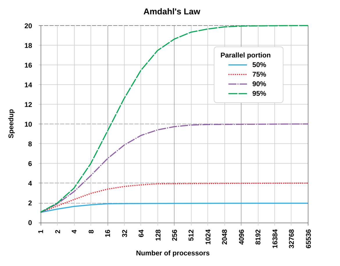
Amdahl’s Law in action: Speedup vs. number of processors for workloads with 50%, 75%, 90%, and 95% parallelizable content. Even with thousands of processors, the speedup plateaus due to the serial portion (the horizontal dashed lines show the theoretical limit for each case). This illustrates the diminishing returns of adding more parallel units.

The Parallelism Bottleneck: Why More Cores Isn’t Always Better

In principle, parallel computing sounds like a ticket to unlimited performance—just keep adding CPUs/GPUs and things run faster. In practice, Amdahl’s Law asserts a hard cap: beyond a certain point, extra processors contribute almost nothing because the task spends most of its time in the unavoidable serial part. This manifests as diminishing returns: going from 1 to 4 processors might yield a big boost, but going from 64 to 128 yields a much smaller percentage gain if the serial fraction dominates. As one industry expert put it, “You can’t just keep scaling processors infinitely and get infinite [speedup]. It just doesn’t work that way anymore.” Eventually, adding cores is like adding more engines to a car that’s stuck in traffic—the constraint isn’t the horsepower, it’s the single-lane road ahead.

Real-world parallel programs also face overhead that effectively increases the serial portion. Tasks running in parallel must often coordinate with each other—merging results, synchronizing steps, communicating over networks or shared memory. These overheads (communication delays, synchronization waits, I/O bottlenecks) all count as “non-parallelizable” work that degrades the payload performance of a parallel system. In an influential analysis, János Végh notes that in any parallelized computing system, activities like inter-process communication and synchronization “are summed up as ‘sequential-only’ contribution” to execution time. The more nodes or threads you have, the more these overheads can grow, eating into the gains of parallelism. Thus, the true speedup in practice might be even lower than the ideal S(N) given by Amdahl’s formula, because Amdahl’s Law assumes perfect parallel efficiency with zero overhead (an assumption that rarely holds at scale ).

This bottleneck isn’t just a theoretical worry; it’s evident in high-performance computing (HPC) benchmarks. A supercomputer might boast a peak throughput of exaFLOPs (10¹⁸ operations/sec) by virtue of massive parallelism, yet its real performance on certain complex workloads is a tiny fraction of that. For instance, when running the High Performance Conjugate Gradients (HPCG) benchmark (which is more communication-heavy) on top supercomputers, the achieved performance can be orders of magnitude lower than peak, essentially “hitting the wall” much sooner than one would expect. In essence, Amdahl’s Law (for a fixed problem size) taught computer architects to be wary of strong scaling limits: beyond some number of processors, you get little bang for your buck. This realization historically influenced system design – for example, even as supercomputers grew in the 1970s and ’80s, there was skepticism about massive parallelism until researchers like John Gustafson argued for scaling up the problem size with the number of processors (known as Gustafson’s Law) to mitigate Amdahl’s fixed-workload assumption. Still, the fundamental point stands: some part of the computation is sequential, and that part becomes the performance ceiling.

AI and Other Demanding Workloads Under Amdahl’s Shadow

The resurgence of artificial intelligence and deep learning in recent years has led to a gold rush in parallel computing – we now train neural networks on hundreds or thousands of GPU cores in parallel. Yet, even AI workloads run up against Amdahl’s Law constraints. Neural networks are often touted as “embarrassingly parallel” during training (since computations for different data samples or layers can be done concurrently), but not everything scales perfectly. There are portions of the training loop that are sequential or require synchronization: aggregating gradients, updating weights, handling input/output, or portions of code that are not GPU-accelerated. As you increase the number of GPUs, these bottlenecks and coordination costs (like the all-reduce operation to average gradients across nodes) start to dominate, reducing the efficiency of scaling. Many teams observe near-linear speedup up to a point, after which adding more GPUs yields diminishing returns – or even no improvement if the communication overhead outruns the computation gains.

Academic research confirms this intuition. Végh (2019) analyzed the performance limits of large-scale neural network simulations and concluded that they “have computing performance limitation” due to the inherently sequential aspects of today’s computing paradigm, as described by Amdahl’s Law. In other words, even though neural networks themselves are massively parallel structures in theory, our processor-based simulators (whether software on CPUs/GPUs or even specialized hardware) still operate with a clock-driven sequential core that forces certain steps to serialize. The result is that scaling up neural network models to more chips yields less and less benefit; at extreme scales, the paper argues, only marginal performance improvements can be expected without a fundamental change in approach. This is one reason why simply throwing more GPUs at tasks like full brain simulation or giant AI models is not a sustainable path to real-time performance – the 70-year-old von Neumann architecture and its sequential choke points become the limiter.

Other data-intensive or scientific workloads exhibit similar behavior. Big data analytics pipelines, weather/climate simulations, financial modeling – they all have components that don’t parallelize well (e.g., a final aggregation step, a time-stepped iteration that needs the previous step’s result, etc.). In such cases, organizations building out large clusters find that beyond a certain cluster size, utilization drops off. Engineers start asking questions like “Where is the limit? What are the problems?” when they see that adding more servers doesn’t linearly decrease runtime. It often turns out the bottleneck has shifted: maybe the network is saturated, or the algorithm spends 90% of its time in a single-threaded section that no GPU can accelerate. As one analyst noted about AI models, performance is about the whole system, not just the number of processors – memory and I/O can bottleneck too, and “there are going to be limitations in the throughput that any given piece of hardware can achieve.”

The implications are clear: for AI and other high-performance tasks, classical computing must confront Amdahl’s Law. We can either (a) live with the ceiling it imposes, meaning accept diminishing returns and seek other ways to improve (like algorithmic efficiency), or (b) find ways to reduce that serial fraction (1–f) by moving more of the work into parallel hardware or otherwise changing the game. This brings us to the strategies that have emerged to push against these limits.

Pushing the Limits: Specialized Accelerators and Smarter Algorithms

While Amdahl’s Law sets an upper bound for a given workload on a given computing model, we’re not entirely helpless. Over the decades, researchers and engineers have developed creative ways to extend performance:

Specialized Hardware Accelerators: One way to reduce the impact of the serial portion is to speed it up dramatically with custom hardware, or to offload more of the workload into parallel units that handle it efficiently. A great example is the rise of domain-specific accelerators in AI. Google’s Tensor Processing Unit (TPU), for instance, is an ASIC designed specifically for neural network operations. By using a massive array of multiply-add units for matrix math, a first-generation TPU ran inference 15× to 30× faster than contemporary CPUs or GPUs, and delivered 30× to 80× higher performance per watt. Such accelerators effectively shrink the T_s and T_p of certain tasks by brute-force speed, and they excel at the parallel part of the workload (e.g. matrix multiplications) far beyond what a general-purpose processor could do. Similarly, GPUs themselves are a form of specialized hardware that turned the tide when single-core CPU speeds plateaued – their hundreds of cores shine on data-parallel tasks like graphics and deep learning. Even FPGAs and custom pipeline processors are used to accelerate streaming data flows or signal processing, ensuring that less time is spent in the “would-be serial” portion on a CPU. The key, however, is that hardware alone can’t eliminate Amdahl’s serial bottleneck – it can only make every part of the program faster, hoping to alleviate the slow spot. If a part of the task truly can’t be parallelized, putting it on faster hardware helps, but only up to the limit; if 10% remains serial, you still can’t exceed 10× overall speedup, no matter if that 10% runs on a CPU or an FPGA. As experts caution, simply moving a function from software to hardware doesn’t help unless that function can be done in parallel or concurrently.

Neuromorphic Computing: An intriguing branch of specialized architecture is neuromorphic computing – hardware modeled after the brain. Neuromorphic chips (such as IBM’s TrueNorth or Intel’s Loihi) implement networks of spiking neurons in silico, running many small, asynchronous events in parallel with minimal centralized control. The brain doesn’t have a single clock driving all neurons each step; neurons fire independently. Likewise, neuromorphic hardware aims to remove the global clock and allow a flood of operations to happen in parallel, which could bypass some sequential bottlenecks. Early neuromorphic systems have shown promise in energy efficiency gains – e.g. using spiking neuron models can improve efficiency for certain AI computations – though they haven’t yet demonstrated speedups on large-scale tasks that outclass GPUs. Nonetheless, the neuromorphic approach represents “thinking outside the von Neumann box”: by emulating brain-like parallelism and event-driven processing, it could avoid some overheads of conventional processors and potentially handle AI workloads with fewer sequential choke points. In practice, neuromorphic computing is still emerging, and current designs often end up integrating with traditional computing workflows (inheriting some limitations of today’s algorithms and training methods ). But it’s a path being explored to keep pushing performance when traditional scaling falters.

Optimized Algorithms and Parallel Models: Perhaps the most powerful lever is improving the algorithms themselves. Amdahl’s Law assumes a fixed problem size and fixed fraction of parallel work, but what if we change the workload or algorithm? High-performance computing practitioners often use Gustafson’s Law, which posits that if you increase the problem size with the number of processors, you can achieve near-linear scaling because the parallel portion grows with N (this is “weak scaling”). In simpler terms, instead of asking “How fast can I solve this fixed problem with more processors?”, ask “How much larger a problem can I solve in the same time with more processors?” – which often yields a more optimistic answer. Algorithmic innovations can also decrease the serial fraction or the overall work. For example, replacing a sequential algorithm of complexity O(N) with a parallel divide-and-conquer algorithm that is largely O(log N) sequential and O(N) parallel can drastically increase f. Even outside of parallelization per se, improvements in algorithms (say going from quadratic complexity to linear complexity) can yield far bigger gains than hardware scaling. In AI, researchers develop better distributed training algorithms that overlap communication with computation, reduce synchronization frequency (like stale gradient updates or asynchronous methods), or compress the exchanged data to reduce communication. All these techniques aim to minimize the sequential component or the overhead, effectively pushing the boundaries that Amdahl’s Law would otherwise impose. In industry, there’s a constant effort to “make the algorithms more efficient” and limit things like bandwidth usage and synchronization so that hardware can be kept busy doing parallel work. One current example is the work on model parallelism and pipeline parallelism for training gigantic neural networks – instead of one big layer that can’t be split (which would be a serial part when scaling data parallelism), engineers split models across devices and pipeline the execution so multiple batches are in flight. This doesn’t defy Amdahl’s Law, but it redistributes the workload to maximize parallel activity and keep the serial fraction as small as possible.

Each of these approaches – faster domain-specific hardware, neuromorphic design, and algorithmic breakthroughs – has pushed the envelope of classical computing. We’ve managed to continue performance growth despite the slowdown of Moore’s Law largely thanks to parallelism and specialization. Yet, all these are still fundamentally within the realm of classical computing. They can extend the frontier, but they don’t break the ultimate rule that a certain amount of the process is sequential on a classical Turing machine model. To truly go beyond, we might need a different kind of computation altogether. This is where many look to quantum computing.

A Quantum Leap: How Quantum Computing Differs and Dodges Amdahl’s Law

Quantum computing offers a radical departure from classical parallelism. Instead of many processors executing chunks of a task concurrently, a quantum computer leverages quantum parallelism – the ability of quantum bits (qubits) to exist in a superposition of states – to explore many possibilities at once within a single computational process. In essence, a quantum processor is not splitting one problem into many smaller sub-problems run by separate cores; rather, it operates on a superposed state space that encodes many potential solutions simultaneously, and uses quantum operations (unitaries and measurements) to interfere those possibilities and extract an answer. As researchers describe it, “a quantum computing core is inherently an elementary parallel computing unit: calculations can be performed in parallel by unitary transformations acting on a superposition of quantum states.” In other words, with N qubits you have 2^N basis states, and a quantum operation can in one step affect all of those components of the superposition. That’s an exponential parallelism baked into the physics of the machine, rather than requiring exponential physical hardware.

Crucially, this kind of quantum parallelism doesn’t map neatly to Amdahl’s framework of “parallel fraction f vs serial fraction 1–f.” Amdahl’s Law assumes we are performing the same algorithm faster by parallelizing parts of it across multiple identical processors. Quantum computing instead often achieves speedups by using different algorithms that leverage quantum mechanics. For certain problems, quantum algorithms can reduce the complexity so dramatically that it outpaces any classical speedup achievable by Amdahl’s incremental approach. A famous example is Shor’s algorithm for integer factorization. Classically, the best known factoring methods run in super-polynomial time (sub-exponential in some cases, but effectively intractable for large numbers). Shor’s quantum algorithm can factor numbers in polynomial time, e.g. factoring an L-bit number in roughly O(L³) steps. This isn’t just a constant or linear speedup – it’s an exponential speedup over the best known classical approach. As one paper’s abstract put it, “Shor’s algorithm for factoring in polynomial time on a quantum computer gives an enormous advantage over all known classical factoring algorithms.” In terms of impact: a problem that might take millions of years on classical machines could in principle be done in hours on a quantum computer, because the quantum algorithm isn’t constrained by plodding through one candidate at a time or even a million candidates in parallel – it finds structure (like periodicity in Shor’s algorithm) via quantum interference that shortcuts the brute-force process entirely.

It’s important to note that quantum computers do not simply make everything faster; rather, they excel on certain problems by exploiting mathematical structures with quantum phenomena. For problems that have known efficient classical solutions, a quantum computer may not offer much advantage. But for a class of problems, quantum algorithms fundamentally outpace classical ones. Another well-known example is Grover’s algorithm for unstructured search, which provides a quadratic speedup (it finds a target item in an unsorted database of size N in O(√N) steps, whereas classically it’s O(N)). Quadratic is not as mind-bending as exponential, but it’s still a different scaling than any classical parallelization can achieve for the same problem. If you threw N processors at the search problem classically (one checking each item), by Amdahl’s reasoning you could achieve at best a linear speedup (N processors → N times faster, so O(N/N) = O(1) expected time, which is fine for search). But quantum does it with far fewer “hardware” resources (one quantum processor acting in superposition) and achieves a result in significantly fewer steps than any classical algorithm running on any number of processors would require.

The key distinction is that quantum parallelism is not the same as classical parallel processing. Quantum computing doesn’t run many threads in parallel; it evolves a complex quantum state that represents many computational basis states in superposition. As long as the problem can be encoded such that the correct answer can be extracted via interference of those states, the quantum computer isn’t limited by a single “serial” bottleneck in the same way. There is still a form of sequential step – for instance, quantum algorithms have sequences of operations, and ultimately reading out the answer (measurement) is a physical act that yields one result at a time. In fact, some computer scientists have examined how laws like Amdahl’s might translate (or not) to quantum. A recent conference paper pointed out that classical parallelism laws offer insights but “their direct application to quantum computing is limited due to the unique characteristics of quantum parallelism, including the role of destructive interference and the inherent limitations of classical-quantum I/O.” In simpler terms: you can’t directly apply Amdahl’s formula to a quantum computer because the model of computation is fundamentally different – interference can cancel out wrong answers and amplify right ones in a way that no amount of classical processors working in parallel can mimic, and the bottlenecks often lie in how you input and output data to the quantum machine rather than a portion of the algorithm being serial.

Another way to see it: Suppose you have a problem where 90% of the work is perfectly parallelizable, 10% is serial – Amdahl would cap you at 10× speedup on classical hardware. A quantum computer might attack the problem in a completely different way such that it doesn’t have an analogous “10% serial part” at all; it might solve the whole problem in one stroke of a quantum algorithm. The notion of complexity class is relevant: many researchers are excited about quantum computing because it appears to break the hierarchy assumed by classical computation limits (hence why quantum supremacy demonstrations are milestones). Google’s 53-qubit Sycamore chip famously performed a specialized computation (random quantum circuit sampling) in about 200 seconds, which was estimated to take Summit (one of the world’s fastest supercomputers) around 10,000 years to replicate. Even if that specific task isn’t directly useful, it’s a proof-of-concept that quantum devices can leap far beyond classical HPC for certain problems. To frame it in Amdahl terms: no amount of parallel threads on Summit could achieve that feat in any reasonable time, because the classical algorithm for that task is just exponentially hard. Quantum found a way to do it by essentially leveraging physics to shortcut the computation.

Quantum Computing: The Best Hope to Break the Ceiling?

Given the stark differences outlined, many experts view quantum computing as the most promising path to overcome the classical limits exemplified by Amdahl’s Law. Quantum computers, in theory, won’t be bounded by a fixed serial fraction in the same way – if a problem is in the class that admits a quantum speedup, a sufficiently large quantum computer could blow past the speedup limits of any classical computer, no matter how many cores the classical one has. This doesn’t mean quantum computers will replace classical ones for all tasks (indeed, for lots of everyday computing, classical is perfectly fine or even better). But for the grand challenge problems that strain current supercomputers – cryptography, complex optimization, simulating quantum chemistry and materials, large-scale AI optimization, etc. – quantum algorithms offer a way forward when classical scaling runs out of steam.

One can think of it this way: The last few decades of computing have been about parallelizing our way to higher performance (multicore CPUs, GPUs, clusters, cloud computing). We kept the basic computing paradigm the same (still step-by-step logical operations), but just did more in parallel. Amdahl’s Law was the speed limit sign on this highway. Now, quantum computing is like opening up a whole new highway – one that runs on completely different physical principles (superposition, entanglement) and potentially has a much higher speed limit (for certain problem domains, maybe no practical limit at all short of the size of the quantum computer). It’s not just adding lanes, it’s a different kind of vehicle altogether.

To make a strong case for quantum: consider problems like breaking RSA encryption (factorization) or simulating a molecule precisely. With classical computing, even if you use the entire power of a global cloud datacenter, these tasks might be infeasible in a reasonable timeframe. Amdahl’s Law says even if 99.9% of the task parallelizes, that 0.1% serial part (or just the sheer scale of operations needed) keeps it out of reach. Quantum computing, by changing the algorithmic complexity class, can bring these tasks into reach. If large-scale, error-corrected quantum computers become a reality, we could see breakthroughs such as real-time cryptanalysis, simulation of new pharmaceuticals or materials at the quantum level, and AI optimization routines that find better solutions faster. These are things that would mark not just an incremental step but a qualitative leap in our computational capabilities.

Of course, it’s important to temper the excitement with reality: today’s quantum processors are still small (tens or a few hundred qubits at most) and error-prone. We are in the early days, akin to where classical computing was in the 1940s or 1950s – the devices exist, but they are limited and specialized. The broader computing industry views quantum as a co-processor model in the foreseeable future: we’ll likely have hybrid systems where classical computers handle what they’re good at, and offload quantum-suited sub-problems to a quantum processor (much like GPUs accelerate graphics/AI today). In those hybrid systems, one might say Amdahl’s Law still applies at the top level: if only part of your workload can go quantum and the rest remains classical, that classical part is your new bottleneck. However, the hope is that for really hard problems, the part that dominates runtime classically is the part a quantum computer would handle, drastically reducing the overall runtime. For example, in a drug discovery simulation, maybe 90% of the time in a classical supercomputer is spent calculating quantum chemistry interactions – offload that to a quantum computer which does it exponentially faster, and suddenly the whole task is orders of magnitude faster even if the remaining 10% (setup, data movement) stays classical.

Conclusion: Embracing a Future Beyond Classical Limits

The implications of quantum computing adoption are broad and profound. In the near term, it means reimagining algorithms and software to work in concert with quantum devices – a new paradigm of quantum algorithms and hybrid quantum-classical workflows. It means that some longstanding software assumptions (like certain problems being effectively unsolvable due to time constraints) might no longer hold, which could upend fields like cryptography (necessitating new encryption schemes safe against quantum attacks) and optimization. From a high-level view, if quantum computing delivers on its promise, it will extend the trajectory of computational progress far beyond the flattening curves imposed by Moore’s Law and Amdahl’s Law on classical tech. We could continue to tackle ever larger problems in science and engineering that today would be considered impractical.

However, reaching that future requires significant investment and research now: building quantum hardware at scale, inventing error-correction techniques, and training a generation of engineers fluent in quantum thinking. The intellectual shift is akin to the shift to parallel programming decades ago – developers had to learn to think about concurrency; in the quantum era, they’ll have to learn to think about superposition and probability amplitudes.

In summary, Amdahl’s Law teaches us a humbling lesson about the limits of classical computing: there is always a portion that resists parallel speedup, chaining us to diminishing returns. We’ve coped by clever engineering – making that chain as short as possible – but not broken it. Quantum computing offers a bolt cutter for certain chains, freeing us from some of the constraints that have started to stall high-end computing. It fundamentally changes the rules of the game by leveraging physics in ways classical computers cannot. While classical computing will remain indispensable, the advent of practical quantum computers would mark the beginning of a new epoch in computing – one where “the impossible” starts to become possible, and where the phrase “exponential time” shifts from meaning infeasible to entirely doable in the quantum realm.